How to change the legend name in clustered columns chart in Excel
I am trying to update the legend name presented in a clustered columns chart that I create via a pivot table. There are few ways recommended online how to update the legend name for regular chart types.
For example, in Microsoft's website, this link shows some steps. However, none of these steps are applicable for clustered columns. When I click Select Data, the editing option is not clickable as shown below.
In short, I would like to update the legend name, which is Total in the image shared.
1 Answer
When there is no field in Legend (Series) area, only a single series in pivot chart, its legend name is "Total" by default, and we could not modify it.
Here is a workaround, I hope it could help you.
- Select the Pivot Table > click PivotTable Analyze > Fields, Items & Sets in Calculations Group > Calculated Field, create a calculated field with 0. I named it as "Helper".
Besides, select M1 (Sum of Score) in pivot table, modify it in formula bar as your needs, which would be the legend name in pivot chart. I want to name it as "Score", but it has been existed, so I need to add a space before it.
- Drag this field into Values area, then you would get the chart as below one.
- Right click "Values" button > Choose "Hide All Field buttons on chart".
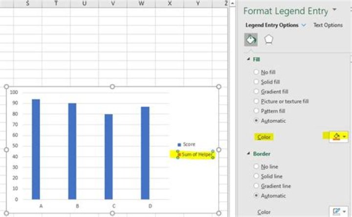
- Set all white for the extra legend (Sum of Helper), including Fill and Text.
- The last result is the following picture.