Can someone intuitively explain what the convolution integral is?
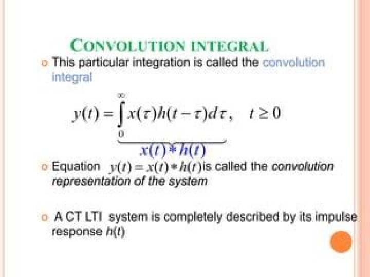
I'm having a hard time understanding how the convolution integral works (for Laplace transforms of two functions multiplied together) and was hoping someone could clear the topic up or link to sources that easily explain it. Note: I don't understand math notation very well, so a watered-down explanation would do just fine. $$(f * g)(t) = \int_0^t f(\tau)g(t-\tau)\ \mathrm{d}\tau$$
This is what my textbook has written. What do those lowercase t-like symbols represent (I haven't seen them before).
$\endgroup$ 56 Answers
$\begingroup$Intuitively speaking when you are given two signals/or functions $f$ and $g$. You time reverese one of the signals, it doesnt matter which one, and shift it by a value of $t$ then you simply multiply and then sum the area under the intersection.
If you consider a function say function of $x$, then time reversal means inserting $-x$ wherever you see $x$ in this function.
Example:
Question1: Assume you have a function $f(x)$ that is $1$ if $x\in[0,1]$, and $0$ elsewhere then how should you plot $f(-x)$?
Question2: Assume you have $g(x)=f(x)$ is there any intersecting area between $f(x)$ and $g(x)$?
Question3: Now shift $g(-x)$ by $0.5$, that is to find $g(-x+0.5)$. How does it look like when you plot it?
Question4: Where does the intersecting region lie in this case $x\in?$ what is the are of the intersecting region? Answer: below white area$=0.5$ at $x=0.5$ shift.
Question5: If you select the shifting parameter not $0.5$ but all reals in $[0,2]$ what function should you get at the output? check $x=0.5$ and see $f*g(x)$ is $0.5$ as found at step 4
EDIT: You define convolution integral in $[0,t]$ for bounded signals. The integral limits depend on where your signal is non-zero.
If you have two signals as you suggested $f(t)=e^{at}$ and $g(t)=e^{bt}$ then the first question: what is the relation between $a$ and $b$? are they positive? where is the function defined? For example when $a$ and $b$ are some positive terms then we have the following integral
$$h(t)=\int f(\tau)g(t-\tau)d\tau= \int e^{a\tau}e^{b(t-\tau)}d\tau=e^{bt}\int e^{(a-b)\tau}d\tau=\Bigg]_{\tau\in\Omega}\frac{e^{(a-b)\tau}}{a-b}$$
clearly $\Omega=\mathbb{R}$ is not possible because the integral does not converge.
$\endgroup$ 2 $\begingroup$I believe the convolution functions makes the most sense when you see it applied in probability theory.
Let X and Y be two random variables and f(X) and g(Y) be the probability distributions of the random variables.
Then the distribution of the sum of two random variables:
$$ (f*g)(t) = \int^t_0 f(-\tau)g(\tau - t )d\tau $$
Why is this? Let us visualize the simple case of rolling dices. and X be the outcome of the first roll and Y be the outcome of the second roll. What is the distribution of the sum?
Since our distributions are discrete, $$ (f*g)(t) = \sum^t_{i=0} f(t)g(i-t) \quad t\in[2,12] $$ This basically translates to, sum up all probabilities such that it has this probability.
i.e. $$(f*g)(4)= \sum^4_{i=0} f(t)g(i-t) =f(1)g(3) + f(2)g(2)+ f(3)g(1) = 1/12 $$
Which is the answer we expect. We can also look at the question from a more physics point of view where it is a time reversed signals but I find this much more intuitive.
$\endgroup$ 2 $\begingroup$Consider the sequences $x_0, x_1, \dotsc$ and $y_0, y_1, \dotsc$.
Now, $$ \left( \sum_{j=0}^n x_j \right) \left( \sum_{j=0}^n y_j \right) = \sum_{z=0}^n z_j, $$ where $$ z_j = \sum_{k=0}^j x_k y_{j-k}. $$
$\endgroup$ 2 $\begingroup$If you want a broad overview, the convolution "blends" two functions together & is the expression of the amount of overlap of one function as it is shifted over another. The convolution takes two functions (& one of them may be a kernel). Writing one of them as a translation, multiply them together & they give you a new function that takes the best properties of both functions. If you take a kernel (as I mentioned above) the new function may have properties from that kernel. A good example would be from something I am interested in: Littlewood-Paley theory. When embarking on various LP constructions, we end up with LP operators such as
\begin{equation*} \Delta_j(f)=\Delta^{\Psi}_{j}=\Psi_{2^{-j}}\ast f. \end{equation*}
These have been defined by constructing a partition of unity (where we are constructing results locally & extending them globally) where $\Psi$ is a radial Schwartz function on $\mathbb{R}^n$ with certain support properties.
Looking at the convolution, $\Delta_j(f)$ has properties that $f$ had as well as support properties passed onto it from $\Psi.$
$\endgroup$ $\begingroup$Intuition for Convolution
A convolution is an amount of overlap of one function f as it is shifted over another function g at a given time offset.
Let’s say we are transforming a certain function f(t) by passing it through a filter g(t) to get the output h(t):
f(t) -> [ g(t) ] -> h(t)Say f(t) has the following values for t = [1, 2, 3, 4, 5] -> f(t) = [1, 2, 3, 4, 5], and
say g(t) has the following values for t = [1, 2, 3] -> g(t) = [3, 2, 1]
Now the question is what is the value of h(t) at a specified time t.
To find the value of h(t) at any time t, let's start with following -
Idea:
Imagine flipping the f(t) with respect to time values, because that is
what it looks like when it enters the filter [g(t)]
Now let's start here,
->| start of time (t) [1, 2, 3] -> time f(t) = [5, 4, 3, 2, 1] g(t) = [3, 2, 1]To calculate the values of h(t), let’s line up the values of f(t) and pass them through the values of g(t)
At t = 1
 g(t) 3 2 1 f(t) 5 4 3 2 1
Total value 3 <-(3x1) = 3
At t = 2
 g(t) 3 2 1 f(t) 5 4 3 2 1
Total value 6 2 <-(3x2)+(2x1) = 8
At t = 3
 g(t) 3 2 1 f(t) 5 4 3 2 1
Total value 9 4 1 <-(3x3)+(2x2)+(1x1) = 14
At t = 4
 g(t) 3 2 1 f(t) 5 4 3 2 1
Total value 12 6 2 <-(3x4)+(2x3)+(1x2) = 20
At t = 5
 g(t) 3 2 1 f(t) 5 4 3 2 1
Total value 15 8 3 <-(3x5)+(2x4)+(1x3) = 26
At t = 6
 g(t) 3 2 1 f(t) 5 4 3 2 1
Total value 10 4 <-(2x5)+(1x4) = 14
At t = 7
 g(t) 3 2 1 f(t) 5 4 3 2 1
Total value 5 <-(1x5) = 5
Just by sliding to any t = n, we can find the value of h(t) by calculating the value of overlapped “area” at t = n.
Now the value h(t) = conv(g(t), h(t)) at any time t is as follows
 g(t) * f(t) = h(t)
[3 2 1] * [1 2 3 4 5] = [3 8 14 20 26 14 5] 1 2 3 4 5 1 2 3 4 5 6 7Note:
So far we have been doing a simple summation of terms as our functions are discrete, if we are dealing with continuous functions the integral as a limit of a summation would come into play.
If you have Matlab, please see
Credit: The above example is based on the Intuitive Guide to Convolution @ Better Explained
$\endgroup$ $\begingroup$This is quite late to the party but here is another (in my opinion very useful) way to look at the convolution integral: changing frames of reference in Quantum Mechanics.
Suppose I have a quantum particle $P_1$ whose location relative to a fixed observer $O$ is given by a probability distribution $p_1(x,t)$ (here $x$ is a real number, basically a coordinate on a line) such that given a set of locations $D$ on the line at a particular time $t_s$ the probability of finding the particle in the location $D$ is given by
$$ \int_{D} p_1(x,t_s) dx $$
To be concrete in our 1 dimensional example we might ask "what is the probability of finding the particle in the interval from $x=1$ to $x=5$?" and we would find this by evaluating
$$ \int_{1}^{5} p_1(x,t_s) dx $$
(for people with a physics background $p_1(x,t) = |\Psi_1(x,t)|^2$).
Now suppose I have another particle $P_2$ whose location relative to the fixed observer $O$ is given by a similar probability distribution $p_2(x,t)$.
It is natural then to ask, what is the relative location of $p_2$ versus $p_1$? For example: "what is the probability that $p_2$ is 3 or more units to the left of $p_1$ at time $t_s$?". In classical mechanics this is easy to do, we just "subtract the frame of reference" but in quantum mechanics this is much trickier (I can elaborate on this if requested in the comments), our desired "frame of reference change" should work as below:
We are looking for a probability distribution function $R(x,t)$ such that if we have a relative space $D$ then
$$ \int_{D} R(x,t_s) dx $$
Gives the probability of $P_2$ and $P_1$ in that relative configuration at time $t_s$. To be concrete we will use the example from earlier:
If we ask "What is the probability that $P_2$ is 3 or more units to the left of $P_1$ at time $t_s$?" then the answer to that must be $$ \int_{-\infty}^{-3} R(x,t_s) dx $$
Now it turns out after all this set up that
$$ R(x,t) = \int_{-\infty}^{\infty} p_2(x-y,t)p_1(y,t) dy $$
Which is just a convolution. So here's yet another application/way to think about the convolution.
$\endgroup$